In order to begin to make a connection between the microscopic and macroscopic worlds, we need to better understand the microscopic world and the laws that govern it. We will begin placing Newton’s laws of motion in a formal framework which will be heavily used in our study of classical statistical mechanics.
First, we begin by restricting our discussion to systems for which the forces are purely conservative. Such forces are derivable from a potential energy function 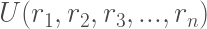
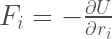
It is clear that such forces cannot contain dissipative or friction terms. An important property of systems whose forces are conservative is that they conserve the total energy

To see this, simply differentiate the energy with respect to time:

noting


This is known as the law of conservation of energy.
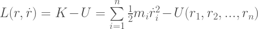
For conservative systems, there is an elegant formulation of classical mechanics known as the Lagrangian formulation. The Lagrangian function, L, for a system is defined to be the difference between the kinetic and potential energies expressed as a function of positions and velocities. In order to make the nomenclature more compact, we shall introduce a shorthand for the complete set of positions in an N-particle system: (

In terms of the Lagrangian, the classical equations of motion are given by the so called Euler-Lagrange equation:

The equations that result from application of the Euler-Lagrange equation to a particular Lagrangian are known as the equations of motion. The solution of the equations of motion for a given initial condition is known as a trajectory of the system. The Euler-Lagrange equation results from what is known as an action principle. We shall defer further discussion of the action principle until we study the Feynman path integral formulation of quantum statistical mechanics in terms of which the action principle emerges very naturally. For now, we accept the Euler-Lagrange equation as a definition.
The Euler-Lagrange formulation is completely equivalent to Newton’s second law. In order to see this, note that


Therefore,
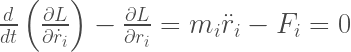
which is just Newton’s equation of motion.
An important property of the Lagrangian formulation is that it can be used to obtain the equations of motion of a system in any set of coordinates, not just the standard Cartesian coordinates, via the Euler-Lagrange equation.
Lagrangian mechanics is a reformulation of classical mechanics, introduced by the Italian-French mathematician and astronomer Joseph-Louis Lagrange in 1788.
In Lagrangian mechanics, the trajectory of a system of particles is derived by solving the Lagrange equations in one of two forms, either the Lagrange equations of the first kind, which treat constraints explicitly as extra equations, often using Lagrange multipliers; or the Lagrange equations of the second kind, which incorporate the constraints directly by judicious choice of generalized coordinates. In each case, a mathematical function called the Lagrangian is a function of the generalized coordinates, their time derivatives, and time, and contains the information about the dynamics of the system.
No new physics are necessarily introduced in applying Lagrangian mechanics compared to Newtonian mechanics. It is, however, more mathematically sophisticated and systematic. Newton’s laws can include non-conservative forces like friction; however, they must include constraint forces explicitly and are best suited to Cartesian coordinates. Lagrangian mechanics is ideal for systems with conservative forces and for bypassing constraint forces in any coordinate system. Dissipative and driven forces can be accounted for by splitting the external forces into a sum of potential and non-potential forces, leading to a set of modified Euler–Lagrange (EL) equations. Generalized coordinates can be chosen by convenience, to exploit symmetries in the system or the geometry of the constraints, which may simplify solving for the motion of the system. Lagrangian mechanics also reveals conserved quantities and their symmetries in a direct way, as a special case of Noether’s theorem.
Lagrangian mechanics is important not just for its broad applications, but also for its role in advancing deep understanding of physics. Although Lagrange only sought to describe classical mechanics in his treatise Mécanique analytique, William Rowan Hamilton later developed Hamilton’s principle that can be used to derive the Lagrange equation and was later recognized to be applicable to much of fundamental theoretical physics as well, particularly quantum mechanics and the theory of relativity. It can also be applied to other systems by analogy, for instance to coupled electric circuits with inductances and capacitances.
Lagrangian mechanics is widely used to solve mechanical problems in physics and when Newton’s formulation of classical mechanics is not convenient. Lagrangian mechanics applies to the dynamics of particles, while fields are described using a Lagrangian density. Lagrange’s equations are also used in optimization problems of dynamic systems. In mechanics, Lagrange’s equations of the second kind are used much more than those of the first kind.
